Tutorial: Analyze spending Habits Using Pivot Tables

Before you build the budget that will help you make all your dreams come true, you need to understand your spending habits. I’m going to walk you through the exact steps you can take to analyze your spending habits using Excel pivot tables.

The goal is to categorize your expenditures into manageable buckets. To isolate expenses that can be reduced via daily decision making and lifestyle changes. In essence, we target the low-hanging fruit that can be managed without changing where you live, what you drive, and where you work. Let’s dive in.

Download Your Transactions

The first step to determine your spending habits is to download your transactions from your bank and credit card accounts. This involves logging into every account and downloading the data into a Excel spreadsheet or CSV file.

While each account has a different look and feel, most banks and credit cards allow you to download your data from their websites. Follow these steps:

1. Log into your account.
2. Navigate to the transaction details page.
3. Look for a download button or icon in the top right corner above the list of transactions.
4. Set your time frame – I recommend 3 or 6 months of data. Whichever you choose, make sure you use that time-frame consistently with each account.
5. Download the data as a csv or Excel file – either will work.
6. Repeat this process for each bank and credit card account.

Each bank’s interface looks a bit different. Here are two examples of what to look for when downloading data:

Ally Bank

Bank of America

Organize Your Data

Start by creating a master spreadsheet that you will use to import data from all of the files you downloaded.

• Open Microsoft Excel
• Save it and name it “Spending Habits”
• Go to File/Open/Browse and then select “All Files” on the dropdown if you have csv files you need to open.

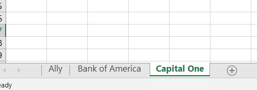
• Open each file, copy the data, and paste it into a new tab in your master spreadsheet. Give each tab the name of the bank or credit card associated with the data.

• After you add data to each tab, the next step is to make the data cohesive. Each dataset will look a bit different. The goal is to combine all of the data onto one worksheet. The only columns you need are Date, Description (it could be called Vendor or another name), and Amount. Create a new tab and add the columns Date, Description and Amount. Name the tab “All Data”.
• Ignore any data you downloaded that doesn’t fit into the Date, Description, or Amount columns. If your data has two amount columns – one for credits to your account and one for charges, create a new column and make the credits positive and the charges negative before you copy it into the “All Data” tab.
• You will need to Paste Values before you copy it if you used formulas. To paste values, right click the highlighted data, Paste Special, and then click the Paste Values radio button.
• Once all of your data is organized into one worksheet under the 3 columns, its time to begin assigning categories.

Categorize Your Data

Choose categories that align with your goal. Your goal is to bucket expenses in a way that you can manage them, and to establish a baseline for your future budget. In business, budgets are based off of prior year income and expense, with new business and growth volumes as “assumptions”, usually in the form of a percent. Expenses that are variable grow in conjunction with volume assumptions, unless there’s an operational change or administrative effort to reduce a certain expense type.

To use this same methodology for creating a personal budget, you need to bucket expenses the same way they would be bucketed on a profit and loss statement. The exception to this is if you have a special type of expense that you struggle with. For instance, if you struggle with eating out too much, you want to segregate restaurant food spending from total food spending to track your future expenses and make them manageable.

So think about your current spending habits. Pick out the three areas you need to work on the most, and will be included in our buckets, even if they normally would have been grouped in another bucket.

This is a standard list of personal finance expense buckets:

• Housing
• Utilities
• Transportation
• Repairs and Maintenance
• Debt Payments
• Childcare
• Medical & Dental
• Food
• Supplies
• Entertainment
• Travel
• Personal Care – clothing, shoes, hair care, etc.
• Other – Tailored to Your Needs
• Other – Tailored to Your Needs

Create a new column called “Category”. At this point I recommend using the Excel sort function to sort your data by description. This will help put similar items together, to make it easier to do the next step.

To sort your data by description, select ALL of it, and then on the Home tab at the top, go to Sort/Filter on the far right and click on “Custom Sort”.

Sort A-Z by Description and choose Order A to Z.

The next step is a cumbersome process, but will save you loads of time in the long run.

In your column you named “Category”, go through each line item in your data set and give it an appropriate category as listed above in this article, or according to how you decided to bucket your expenses. Make sure you spell each category consistently, with the same capitalization used each time.

When you create pivot tables, Excel will only group together items that are identical, so consistency is key to making this process work.

When each expense item has a category next to it, you’ve completed this step.

clean up the Data

Its much easier to work with data when its in the format you need. Most likely, the downloads from the bank and credit card accounts have dates, not months, in the date column. If you want to pivot your data based on Month, you need a Month column. This is way easier to create than you’d think.

Steps to create a “Month” column:

• Highlight the column to the right of your Date column.
• Right click on the letter on top of the column and click “Insert”. This should insert a blank column.
• In the first cell of the blank column, insert this formula:
  • =month(B1) where B is the column where your date is located.
  • Highlight the entire column with your new formula and format as General.

• Double click in the bottom right of the cell with the newly entered formula, and double click to copy it all the way down to the last line of your data OR copy the cell with the new formula, highlight the cells beneath it, and paste it into the cells below.
• The result should be a number correlating to the month of the year associated with your date. For instance, January will be a 1, February a 2, March a 3, and so on.

This will enable us to pivot by month with little effort.

Creating the Pivot Table

Here’s where you leverage the power of pivot tables to slice and dice your data into magic buckets.

Don’t worry if you’ve never created a pivot table in Excel before. I’m going to walk you through the steps.

• First, select all of the columns where you have data. If you used the columns I recommended above, you should select columns A:E.
  1. Date
  2. Month
  3. Description
  4. Amount
  5. Category
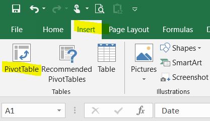
• Go to “Insert” at the top of the screen and then “PivotTable” on the far left.

• Click “Ok” and Excel will create a new tab in your workbook that looks like this:

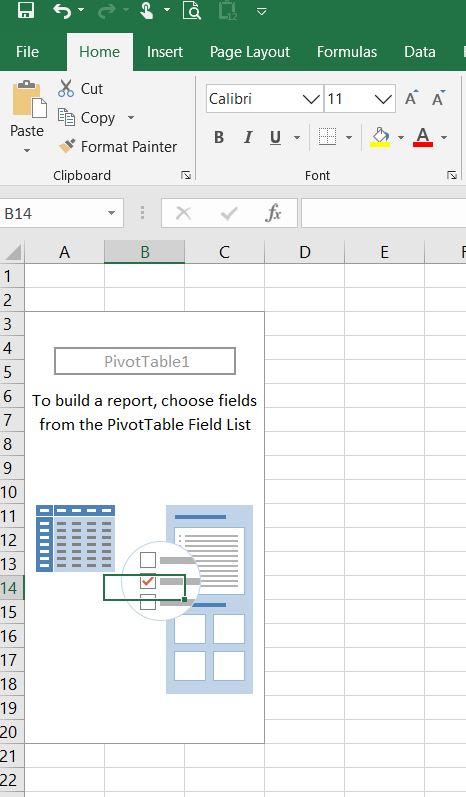
• If you don’t see PivotTable Fields on the right, click into the pivot table and they should appear. Like magic! Pivot table fields look like this:

For an analysis of spending patterns, the goal is to look at expenses by category by month. To do that, drag “Category” into the Rows section, “Month” into the Columns section, and “Amount” into the Values section.

If your Amount values defaults to “Count” instead of “Sum”, click on the drop down arrow to the right of the words “Count of Amount” and click on Value Field Settings. From there you can change from count to sum.

If you have rows or columns that say “blank”, those are either rows you didn’t enter a category for, or they are total lines. Typically you’ll want to filter those out. Go back to your data table and make sure you entered a category for every line item except for totals.

Then go ahead and filter out “blank” by using the drop-down arrow next to Row Lables, and again next to Column Labels.

Click the drop downs and unclick the box next to “blank” to filter them out.

Now look at your expenses by category in your pivot table.

You should have a neat list of income and expenses by category. Now you can properly analyze your data.

What are you spending more money on than you thought? Which areas can you cut back on? Jot down some target amounts next to each category and start planning to decrease your expenses in areas where you have the most opportunity.

Use this pivot table as a guide – a basis – for your budget.

If you update your data table, you can easily update your pivot table as well. Just right click on the pivot table and click on “refresh” to update it.

Congratulations! You now have a baseline for your budget, and valuable information about how much money you can save by cutting back in specific areas of discretionary spending. Your final pivot table should look something like this:

How can you improve your spending habits?